【OpenCV】 ⚠️高手勿入! 半小时学会基本操作 ⚠️ 直线检测
概述
OpenCV 是一个跨平台的计算机视觉库, 支持多语言, 功能强大. 今天小白就带大家一起携手走进 OpenCV 的世界. (第 13 课)

霍夫直线变换
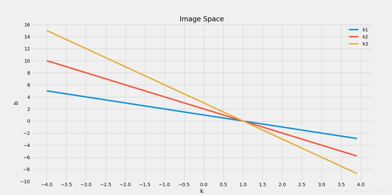
霍夫变换 (Hough Line Transform) 是图像处理中的一种特征提取技术. 通过平面空间到极值坐标空间的转换, 可以帮助我们实现直线检测. 如图:
原理详解
当我们把直线 y = kx + b 画在指标坐标系上, 如下图. 我们再从原点引线段到直线上的任一点.
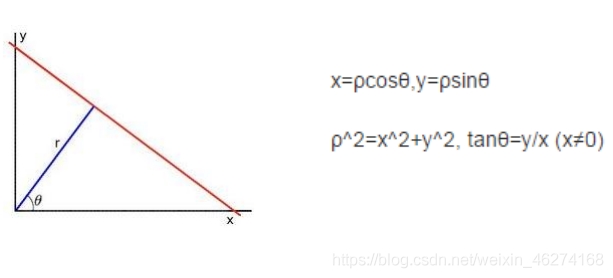
我们可以得到这条线段与 x 轴的夹角为 θ, 距离是 r. 对于直线上的任一点 (x0, y0), 我们可以得到公式:

代码实战
HoughLines
格式:
cv2.HoughLines(image, rho, theta, threshold, lines=None, srn=None, stn=None, min_theta=None, max_theta=None)
参数:
- image: 输入图像
- rho: 线性搜索半径步长, 以像素为单位
- theta: 线性搜索步长, 以弧度为单位
- threshold: 累计阈值
例子:
import numpy as np
import cv2
from matplotlib import pyplot as plt

# 读取图片
image = cv2.imread("sudoku.jpg")
image_copy = image.copy()

# 转换成灰度图
image_gray = cv2.cvtColor(image, cv2.COLOR_BGR2GRAY)

# 边缘检测, Sobel算子大小为3
edges = cv2.Canny(image_gray, 170, 220, apertureSize=3)

# 霍夫曼直线检测
lines = cv2.HoughLines(edges, 1, np.pi / 180, 250)

# 遍历
for line in lines:
    # 获取rho和theta
    rho, theta = line[0]
    a = np.cos(theta)
    b = np.sin(theta)
    x0 = a * rho
    y0 = b * rho
    x1 = int(x0 + 1000 * (-b))
    y1 = int(y0 + 1000 * (a))
    x2 = int(x0 - 1000 * (-b))
    y2 = int(y0 - 1000 * (a))
    cv2.line(image_copy, (x1, y1), (x2, y2), (0, 0, 255), thickness=5)

# 图片展示
f, ax = plt.subplots(2, 2, figsize=(12, 12))

# 子图
ax[0, 0].imshow(cv2.cvtColor(image, cv2.COLOR_BGR2RGB))
ax[0, 1].imshow(image_gray, "gray")
ax[1, 0].imshow(edges, "gray")
ax[1, 1].imshow(cv2.cvtColor(image_copy, cv2.COLOR_BGR2RGB))

# 标题
ax[0, 0].set_title("original")
ax[0, 1].set_title("image gray")
ax[1, 0].set_title("image edge")
ax[1, 1].set_title("image line")

plt.show()
输出结果:


HoughLinesP
此函数在 HoughLines 的基础上末尾加了一个代表概率 (Probabilistic) 的 P, 表明它可以采用累计概率霍夫变换, 来找出二值图像中的直线.
格式:
HoughLinesP(image, rho, theta, threshold, lines=None, minLineLength=None, maxLineGap=None)
参数:
- image: 输入图像
- rho: 线性搜索半径步长, 以像素为单位
- theta: 线性搜索步长, 以弧度为单位
- threshold: 累计阈值
- minLineLength: 最短直线长度
- maxLineGap: 最大孔隙距离
例子:
import numpy as np
import cv2
from matplotlib import pyplot as plt

# 读取图片
image = cv2.imread("sudoku.jpg")
image_copy = image.copy()

# 转换成灰度图
image_gray = cv2.cvtColor(image, cv2.COLOR_BGR2GRAY)

# 边缘检测, Sobel算子大小为3
edges = cv2.Canny(image_gray, 170, 220, apertureSize=3)

# 霍夫曼直线检测
lines = cv2.HoughLinesP(edges, 1, np.pi / 180, 100, minLineLength=100, maxLineGap=10)

# 遍历
for line in lines:

    # 获取坐标
    x1, y1, x2, y2 = line[0]
    cv2.line(image_copy, (x1, y1), (x2, y2), (0, 0, 255), thickness=5)


# 图片展示
f, ax = plt.subplots(2, 2, figsize=(12, 12))

# 子图
ax[0, 0].imshow(cv2.cvtColor(image, cv2.COLOR_BGR2RGB))
ax[0, 1].imshow(image_gray, "gray")
ax[1, 0].imshow(edges, "gray")
ax[1, 1].imshow(cv2.cvtColor(image_copy, cv2.COLOR_BGR2RGB))

# 标题
ax[0, 0].set_title("original")
ax[0, 1].set_title("image gray")
ax[1, 0].set_title("image edge")
ax[1, 1].set_title("image line")

plt.show()
输出结果:


jsjbwy