孟德尔随机化(Mendelian Randomization) 统计功效(power)和样本量计算
1 统计功效(power)概念
统计功效(power)指的是在原假设为假的情况下,接受备择假设的概率。
用通俗的话说就是,P<0.05时,结果显著(接受备择假设); 在此结论下,我们有多大的把握坚信结果的显著性,此时需要用到power来表示这种“把握”。
统计功效(power)的计算公式为 1-β。
说到β,要提一下假设检验中的一型错误和二型错误。
一型错误,用 α 表示,全称 Type-I error;
二型错误,用 β 表示,全称 type-II error;
有个比较经典的图表示 Type-I error 和 type-II error:
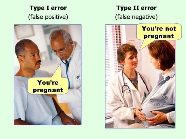
(图片来源忘了,侵删)
因此,Power越大,犯第二型错误的概率越小,我们就更有把握认为结果是显著的。
下面分别从网页版和代码版讲一下怎么计算power和样本量,网页版和代码版均可完成分析,任选其一。
2 网页版计算孟德尔随机化power和样本量
网页版的见地址:https://shiny.cnsgenomics.com/mRnd/
2.1 网页版计算孟德尔随机化power
计算power需要用到7个输入参数,分别为sample size, α, βyx, βOLS, R2xz, σ2(x), σ2(y)。 见下图:
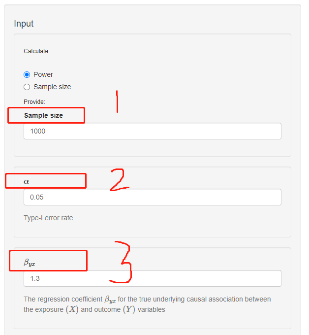
第一个参数sample size,指的是研究的样本量大小;在这里假定样本量是1000;
第二个参数是 α,指的是一型错误(Type-I error),默认0.05;
第三个参数是βyx,指的是暴露变量和结局变量之间 真实 的相关系数。如何理解 真实 呢,以大胸和不爱运动为例,在校正了性别和年龄等一系列可能会影响大胸和不爱运动的变量后得到的回归系数,称为暴露变量(不爱运动)和结局变量(大胸)真实的相关系数;
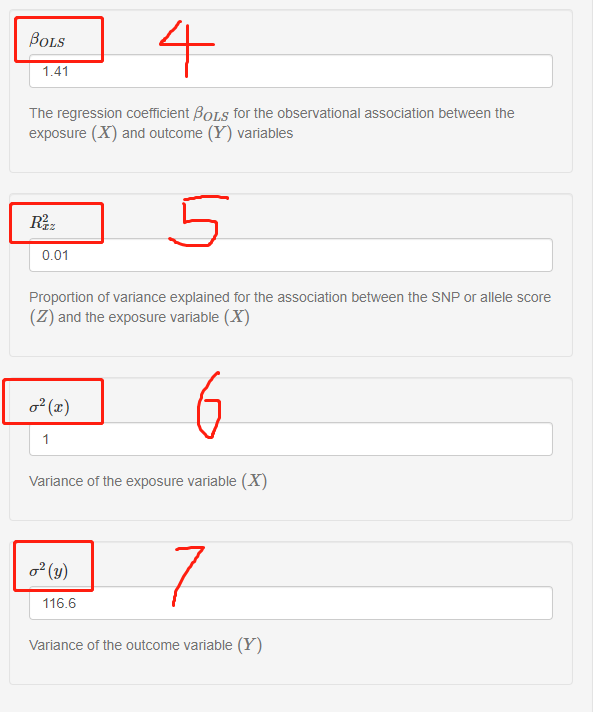
第四个参数是βOLS,指的是暴露变量(不爱运动)和结局变量(大胸)之间 观察到 的相关系数,跟βyx的区别在于,这里不校正协变量;
第五个参数是R2xz,指的是工具变量(一般指SNP)对暴露变量(不爱运动)的解释度;
第六个参数是σ2(x),指的是暴露变量(不爱运动)的方差;
第七个参数是σ2(y),指的是结局变量(大胸)的方差;
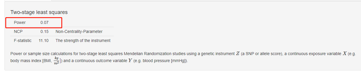
有了这7个参数以后,我们就可以计算power了。 power结果如下所示:
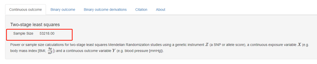
2.2 网页版计算孟德尔随机化样本量
这个步骤同计算power的步骤,唯一不同的是,这个步骤是通过给定power,计算该power下需要的样本量;
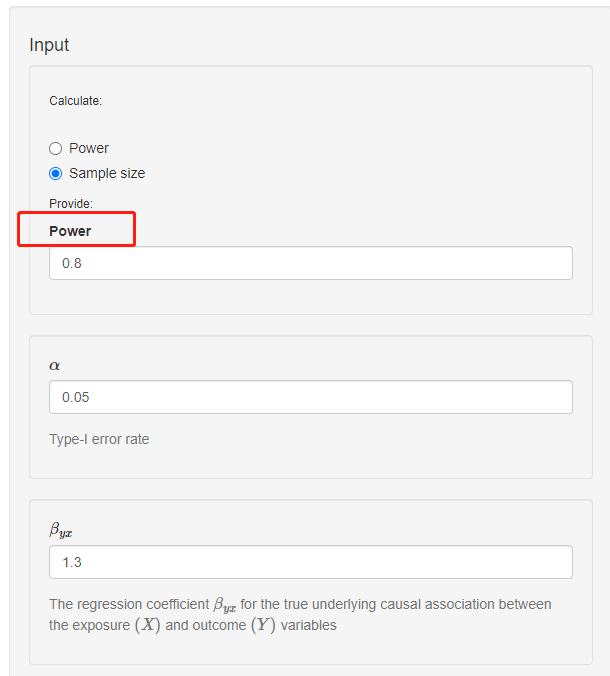
在这里,我们给定的power是0.8,其他的参数同上面的步骤,得到的样本量如下所示:
3 代码版计算孟德尔随机化power和样本量
该代码出自网站:https://github.com/kn3in/mRnd
3.1 代码版计算孟德尔随机化power
在Rscript中运行results函数(以下代码完全照搬,不要修改任何参数):
results <- function(N, alpha, byx, bOLS, R2xz, varx, vary, epower) {

    threschi <- qchisq(1 - alpha, 1) # threshold chi(1) scale
    f.value <- 1 + N * R2xz / (1 - R2xz) #R2xz, Proportion of variance explained for the association between the SNP or allele score (Z) and the exposure variable (X)
    con <- (bOLS - byx) * varx # covariance due to YX confounding
    vey <- vary - byx * varx * (2 * bOLS - byx)

    if (vey < 0) {

        data.frame(Error = "Error: Invalid input. The provided parameters result in a negative estimate for variance of the error term in the two-stage least squares model.")

    } else {

        if (is.na(epower)) {

            b2sls <- byx + con / (N * R2xz)
            v2sls <- vey / (N * R2xz * varx)
            NCP <- b2sls^2 / v2sls
            # 2-sided test
            power <- 1 - pchisq(threschi, 1, NCP)
            data.frame(Parameter = c("Power", "NCP", "F-statistic"), Value = c(power, NCP, f.value), Description = c("", "Non-Centrality-Parameter", "The strength of the instrument"))

        } else {

            # Calculation of sample size given power
            z1 <- qnorm(1 - alpha / 2)
            z2 <- qnorm(epower)
            Z  <- (z1 + z2)^2
            # Solve quadratic equation in N
            a <- (byx * R2xz)^2
            b <- R2xz * (2 * byx * con - Z * vey / varx)
            c <- con^2
            N1 <- ceiling((-b + sqrt(b^2 - 4 * a * c)) / (2 * a)) #ceiling返回对应数字的'天花板'值,就是不小于该数字的最小整数
            data.frame(Parameter = "Sample Size", Value = N1)

        }
    }
}
随后运行以下如下命令:
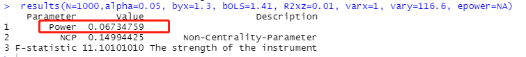
results(N=1000,alpha=0.05, byx=1.3, bOLS=1.41, R2xz=0.01, varx=1, vary=116.6, epower=NA)
各个参数代表的意义如下所示:
alpha=0.05 #Type-I error rate
N=1000 # Sample size
byx=1.3 #the regression coefficients for the association between exposure (X) and outcome (Y) variables (adjusted for confounders).
R2xz=0.01 # genetic instrument that explains R2xz=0.01 of variation in exposure (X)
bOLS=1.41 # the regression coefficients for the association between exposure (X) and outcome (Y) variables (no confounder-adjustment)
varx=1 # Variance of the exposure variable (X)
vary=116.6 #Variance of the outcome variable (Y)
得到的结果如下所示:
3.2 代码版计算孟德尔随机化样本量
该步骤与前面一致,运行results函数后,再运行如下命令:
results(N=NA,alpha=0.05, byx=1.3, bOLS=1.41, R2xz=0.01, varx=1, vary=116.6, epower=0.8)
各个参数代表的意义如下所示:
alpha=0.05 #Type-I error rate
epower=0.8 # 1-(type-II error rate)
byx=1.3 #the regression coefficients for the association between exposure (X) and outcome (Y) variables (adjusted for confounders).
R2xz=0.01 # genetic instrument that explains R2xz=0.01 of variation in exposure (X)
bOLS=1.41 # the regression coefficients for the association between exposure (X) and outcome (Y) variables (no confounder-adjustment)
varx=1 # Variance of the exposure variable (X)
vary=116.6 #Variance of the outcome variable (Y)
得到的结果如下所示:

原文出处:Brion M J A, Shakhbazov K, Visscher P M. Calculating statistical power in Mendelian randomization studies[J]. International journal of epidemiology, 2013, 42(5): 1497-1501.
此推文感谢彭师姐推荐~